Looking for a classical EPR-Bell curve

From where came the EPR Triangle curve?

The so called Triangle curve of the classical correlations is defined as \( c(x)=1-{{2 |x|} \over \pi } \) on the interval \(-{\pi \over 2}\) to \({\pi \over 2}\). c() is the correlations function. How was it found ? What is its origin ? Let’s start a naive analysis to see what we can find after quick and not too much elaborated attempts.

Numerical simulation of the EPR experiment

On each polarizer/arm A and B, a private random angle x is selected and then the probability to be detected is, according to the Malus law, \( f(x)=k Cos^2(x) \) where f() is the Malus-like law and k is the efficiency of the device. Some authors use always k=1 which is unphysical, particularly in QM. Also, the law in cos² is approximative since f(x) is never null , nor equal to k, but close to them at the extrema. Approximatively, \( f(x)= p k Cos^2(x)+g \) where p is another lessening coefficient to better fit the maxima and g the minima.

According to Bell quantum mechanics [1], if x and y are the angles of a given pair, the correlations map must be \( \Delta=x-y , c(\Delta)=Cos^2(\Delta) \). The QM solution assumes that the efficiency coefficient k is equal to 1 and invokes the fair sampling assumption without more details.

Classical mechanics doesn’t provide a turn key solution. As usual, the physicist analyses exactly the setting and searchs a solution based on the known laws. If it is not possible, she tries to establish an emergent law fitting the experimental outcomes before further interpretations. Anyway, she will never use k=1 because there is not any physical context where k=1.

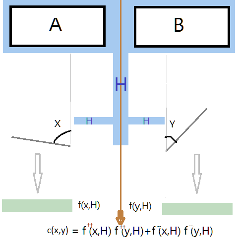
At each trial i, A and B send particles which, according to QM, share the same wave functions. Each polarizer takes secretely a random angle x or y which affects its outcome. If the particle is detected, we record (i,x,+1) else (i,x,0). Because k is never equal to 1, a “0” outcome means “filtered out or loss somewhere“. Indeed, we can observe in the main lab report [2] that the “0” outcome is considerably more frequent than the “1” one. It happens also that experimenters use elaborated devices rendering 1 or -1 or 0 but it is a bad idea in a fundamental experiment to add the assumption that the new devices complex arrangement works as expected.

Reconstructing the real “-1” outcome by symmetry with “1” or doing like if the detection device has also the capacity to answer “-1” is equivalent at the first approximation. For convenience, we will use the latest option. Then, when the detector doesn’t find +1 or -1, it will render “0” and we will record (i,x,0).
When the 2 lists of records are joined on i, we get records like \((i,x,R_x,y,R_y)\), where R is the outcome. The record can now be extended by \(( x-y, R_x R_y )\). The correlations curve will be based on the \(x-y\) differences. \((x,R_x)\) is sufficient to draw the Malus-like curve.

Let’s try a classical analysis with different functions f() and see the resulting shapes of the c() correlations functions computed by Monte-Carlo. The physicality constrains the arm law to have a shape close to the Malus law. Called after the Copenhagen interpretation experiments, the classical mechanics physicist knows that he must find something that shapes in cos². Then it is the goal of this search, somehow similar to the perturbative method. We have one degree of liberty with the Malus law adjustment, another in the way the undetections are accounted.

Without shared variables and without the Malus law

Let’s draw the pure random curve, just to calibrate the simulator and to recall the case.
The independent particles come from different sources. If A and B behaves like random generators rendering always 1 or -1 with a 100% detection rate, their outcomes will correlate in a flat string \(c(x)={1 \over 2}\)

The graphic frame renders

• mainly the correlations curve in green,
• but also the answer for an arm
• and the cross efficiency by degree difference. The cross efficiency is the product of the arms efficiencies.

Malus and QM EPR references curves are in magenta. If they are absent, it means that they are hidden by the computed outcome.

Not possibly physical, the arm law is far from the Malus law. One must always remember that without any link or share, like with 2 independent sources, we get this flat curve in the lab and not the classical Bell curve.

With shared variables but without the Malus law

Another interesting calibration: there is no Malus law, hoping to see it emerging somewhere. The unique argument is the shared variable and then the 2 arms apply exactly the same algorithm. The particularity comes from the Monte Carlo method distribution. The elementary relation is not a function, then final elementary results are not static while their statistics are very stable.

\(f(x) = {Cos^{2}(h)} \\
g(x) = {Sin^{2}(h)} \\
z(x) = { 1 – f(h) – g(h) } = 0 \\ \\\)

Therefore, this leads to a flat curve with 75% of correlations and not 100%. Completely classical and finally 50% better than the quantum curve if correlations high values were usefull.

Not possibly physical, the correlations curve is too far from the experiment outcome. The arm law is also far from the Malus law.

Without shared variables but with the perfect Malus law

It is the typical classical physicist answer when assuming a perfect Malus law. There is not a shared variable to add to the angle.

\(f(x) = {Cos^{2}(x)} \\
g(x) = {Sin^{2}(x)} \\
z(x) = { 1 – f(x) – g(x) } = { 1 – Cos^{2}(x)-Sin^{2}(x) } = 0 \\ \\\)
A very bad curve but also it is not flat and its shape is promising…
Correlations begin to seem physical but they are so far from the experiment outcome. The arm law is exactly the ideal Malus law with k=p=1 and g=0. The efficiency is 100% by construction, since z(x) is always null.

With shared variables and a refined Malus law

Additive shared variables

A shared variable is a broad indication. We notice that we are talking of arguments or arguments modifiers. We know the uncontested approximative real Malus law as \( f(x)= p k Cos^2(x)+g \). It is reasonnable first to look for modifiers of p,k,x and g. Unfortunately, p, k and g are difficult to modify. They might describe the settings. We must likely use 2 modifiers and it is not clear how to do.
x seems to be our target. It is easy to add or substract something and to expect that the means of the statistics will remove any unwished asymmetry. Hence, let’s consider that it is an additive or substractive variable having negative and positive values well distributed around 0. By symmetry, additive or substractive variable are the same. By analogy with the angle differences of the correlations function, let’s use the substraction.

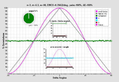
With shared variables and a weakly modified Malus law

As specified, we substract from x a shared variable h well distibuted around 0 within a maximum radius. The distribution seems to the naive.
\(f(x,h) = {Cos^2(x-h)} \\
g(x,h) = {Sin^2(x-h)} \\
z(x,h) = { 1 – f(x,h) – g(x,h) } = { 1 – Cos^2(x-h)-Sin^2(x-h) } = 0 \\ \\\)

oups! It is worst than the naive case: the curves are similar but the Malus law is weird.

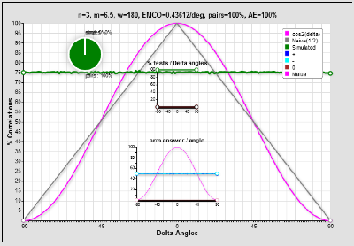
Let’s tinker the above relation

Knowing the \({ 1 – Cos^{2n}(x-h)-Sin^{2n}(x-h) } \) is null when n=1 and positive when n>1, let’s try to see what happens.

\(f(x,h) = {Cos^{2n}(x-h)} \\
g(x,h) = {Sin^{2n}(x-h)} \\
z(x,h) = { 1 – f(x,h) – g(x,h) } = { 1 – Cos^{2n}(x-h)-Sin^{2n}(x-h) } \\ \\\)

The correlations function c of the angles differences c:

\(c(c) ={ {1 \over {2 \rho (\pi -c) }} { \int_{-\pi \over 2}^{{\pi \over 2}-c} {{ \int_{-\rho}^{\rho}
{ { (Cos^{2n}(x-h) \quad Cos^{2n}(x+c-h) \\ + \quad Sin^{2n}(x-h) \quad Sin^{2n}(x+c-h))} } }\quad dh } \quad dx } } \\ \\
\\ \\\)

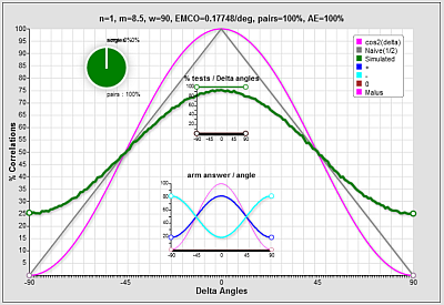
with n=5, we get:

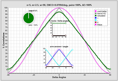
unphysical , it is the Bell classical curve, the Triangle! Did we found the Triangle curve origin? The arm law is far from the Malus law.

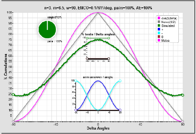
Let’s do a “mistake” with a fair sampling assumption and statistics based on what is detected

Let’s assume again \( n > 1 \) and scale f and g.

\(f(x,h) = {{Cos^{2n}(x-h)} \over {Cos^{2n}(x-h) + Sin^{2n}(x-h)} } \\
g(x,h) = {{Sin^{2n}(x-h)} \over {Cos^{2n}(x-h) + Sin^{2n}(x-h)} } \\
z(x,h) = { 1 -{Cos^{2n}(x-h)} -{Sin^{2n}(x-h)} } > 0 \\\)

The undetected z() probability remains on the emitted number.

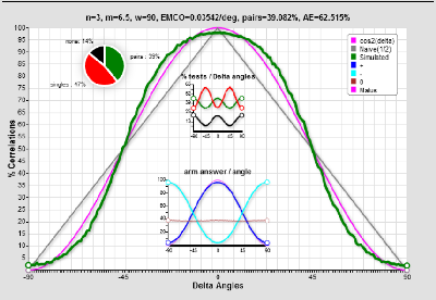
Possibly physical, not so far from the experiment outcome. The arm law is similar to the Malus law. There are better distributions closer to cos² and or with better efficiency. The latter is low, but this curve and a cos² are almost indistinguishable in lab conditions, moreover if the curve is studied only for a very few angles differences.
Try now to write the Bell theorem with this classical reference. Ridiculous!

Better curves

There are many, beginning by the one showed in the specific article. It is possible to distribute the shared variables with a gaussian or to do a more complicated cos² expansion. It is also possible to get better using esoteric behaviors or/and memory but we know that it is unphysical because this would bring too much constraints. In a lot of cases, using memory is equivalent to add shared variables. No one serious sequence treatment might be the generator of the representation of a qbit. It would be another theory with any of the well known consequences.

Conclusion

From where came the “Triangle” curve? It seems that other choices were natural, easy to find and not so different from the quantum outcome.
Trivial propositions make very hard to highlight an experimental difference and can disallow the Bell theorem concept. Why generations of physicists missed this “detail”? On another hand, the “triangle” arises from an analysis similar to the ours. Moreover, it is a particular case of a very efficient generalized Malus law, depending on the experiment settings. What does it mean ? It is troubling.

Anyway,

• To accept scientifically an “action at the distance”, a high precision experiment with a high rate efficiency is still lacking, probably because it is impossible to realize.
• A current better fit exists: just surf on this site and try also the on line simulation!

Reference

1 J. S. Bell (1964) : On the Einstein-Podolsky-Rosen Paradox, Physics 1, 195-200 .
2 Marissa Giustina, Anton Zeilinger et Al: Supplemental Material: Significant-Loophole-Free Test of Bell’s Theorem with Entangled Photons (2013) and Arxiv