by Igael Azoulay
Q-Crypt Project – Paris desk
-
- Abstact :
Lecturers of the Bell experiment always challenge the public to show a better classical function than the so called triangle. The non existence of functions behaving in the way predicted by quantum mechanics is a major condition in the Bell reasonment. We show with simple maths that such functions exist, even in very optimistic lab conditions never really reached by any known fundamental experiment. Starting from the distibutions, we draw the curves for many parameters settings. Moreover, a classical analysis predicts new behaviors of the outcome that might be checked in a lab. Possible other functions exist. Therefore, surprisingly, the Bell analysis in its current version, fails to decide between the Copenhagen and the Einsteinian interpretations of quantum mechanics. - Pdf Version: here
- Abstact :
Summary
-
-
-
- 1. Lab Bell Inequalities Background Express
- 2. Remarks
- 3. One efficient alternative
- 4. Computation by a Monte-Carlo simulation
- 5. About a proof of quantum entanglement using the Bell Settings
- 6. Conclusion
- A Supplemental material
- References
-
-
This article, isolated from other considerations, concerns mainly a proof method. It is intended for all those who are familiar will the Bell experiment and particularly with the curves comparison.
Thought experiments inventors imagine always a perfect sub world, but labs experiments face the problem of the devices sensibilities. In some cases, a presumed perfect thought experiment cannot be transposed in a lab while many try. A small error rate makes difficult to compare the opposed predictions. I shall try to show that this is the case of the Bell experiment here. Henceforth, a lab Bell experiment needs to fulfill more conditions to be conclusive.
1. Lab Bell Inequalities Background Express
The Bell theoretical background, well explained in many books [2], is assumed to be well known.
From a lab point of view, the thought experiment [1] compares the curves of the classical and the quantum correlations.
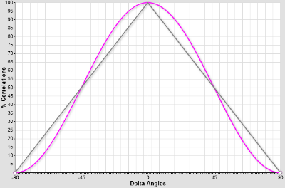
The differences of the angles with the polarizers are the arguments.
The grey curve \( y=1-{{2 |x|} \over \pi } \) represents the classical correlations and the magenta curve y=cos²(x) the quantum correlations.
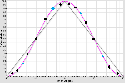
Then, an experiment is conducted, the detections are summed, the correlations counted, the statistics computed with what was detected, the curves drawn and it is observed that it is as expected by QM. In most cases, even in an experiment of importance [4], very few angles are measured, ie the blue dots only, because it was economic at the time the experiment was conceived. By chance, A. Aspect published complete curves [3] and indeed, they are very similar to cos².
It must be noticed that in reports, the Bell correlations are never averaged on the number of emitted particles, but only on the total of detections, at the best case.
To qualify the additional variables, we will prefer the factual “shared” instead of the subjective “hidden”.
Classical correlations and any computational local method assumed being unable to reproduce such measures, the conclusion is that the quantum entanglement is proven.
2. Remarks
2.1 Efficiency
No detector is perfect, particularly in the QM formalism. Lenses, polarizers and devices filter a part of the signals. Therefore, the alternative to + is not necessarily – , it may be also undetected.
If the filtering function changes the distibution, the resulting sample will be unfair. Undetections and unfair sampling open the problem of finding better than this grey classical curve.
Best detectors allow 85 to 90% of efficiency. High quality lenses and devices filter from 10 to 50%. The alternative solution must work with a low level of errors, ie less than 20%. We are talking of real total efficiencies, meaning the ratio detected over emitted. It is the only definition for the detection issue.
2.2 The challenge
Lecturers often challenge the question, paraphrasing A. Aspect when saying “There is the Bell classical curve, let me know if someone has better”. It is reasonable to accept because lab conditions allow a non negligible level of undetections. A nice challenge would be to find a complete cos² curve and not only an expression fitting the 4 or 6 measures needed to establish the Bell inequality with a low undetection rate, lower than the one offered by the best technologies.
3. One efficient alternative
3.1 Arm distribution
Trigonometric functions are sometimes surprising.
I found this distribution of the polarizer answer, a generalization of the Malus law with undetections, which may result of a walk in a crystal. There are many similar distributions and new ones to find.
The arguments are an effective angle x and an other variable h. h is around 0 inside a radius \(\rho\). Three classical states +, – and 0 for “undetected”, which have respectively the probability distributions functions f, g and z depending on x and h. k is an intermediate expression. m and n are free small integers or reals depending on the model of decay or lessening detection. See below in the curves the optimal values for n and m found by trial.
\(k(x,h) = { { (1 – (1 – Cos^{2n}(x-h)-Sin^{2n}(x-h))^m) } } \\f(x,h) = {k(x,h) \quad {{Cos^{2n}(x-h)} \over { (Cos^{2n}(x-h)+Sin^{2n}(x-h))}}} \\
g(x,h) = {k(x,h) \quad {{Sin^{2n}(x-h)} \over { (Cos^{2n}(x-h)+Sin^{2n}(x-h))} }}\\
z(x,h) = { 1 – f(x,h) – g(x,h) } = { (1 – Cos^{2n}(x-h)-Sin^{2n}(x-h))^m } \\ \\\)
With n=1 and m=0 , the distribution becomes the Malus law.
3.2 Correlations
When applying the distribution to 2 polarizers, each one uses only its own local angle x unknown from y and shares the other variable h with the other.
x must be dynamic by construction of the Bell theorem. To work in the solution, h must be dynamic too.
Angles are from \(-{\pi \over 2}\) to \(\pi \over 2\) and the shared variable h is evenly distributed around zero in a radius \(\rho\) from \(0\) to \( \pi\). \( \rho = {\pi \over 4}\) seems interesting.
Let’s compute the correlations of 2 polarizers sharing at each trial the variable h with random x and y, their respective angles. Let’s define \(c = y -x\) , the argument of the correlation function p.
\(P(c,x,h) = { f(x,h) f(x+c,h) + g(x,h) g(x+c,h) } \\= { k(x,h) \quad k(x+c,h) \quad { (Cos^{2n}(x-h) \quad Cos^{2n}(x+c-h) \quad + \quad Sin^{2n}(x-h) \quad Sin^{2n}(x+c-h))} } \\
p(c) ={ {1 \over {2 \rho (\pi -c) }} { \int_{-\pi \over 2}^{{\pi \over 2}-c} { \int_{-\rho}^{\rho}
{P(c,x,h) } \quad dh } \quad dx } } \\ \\
={ {1 \over {2 \rho (\pi -c) }} { \int_{-\pi \over 2}^{{\pi \over 2}-c} \\
{ \int_{-\rho}^{\rho} { k(x,h) k(x+c,h) \\ \quad
{ (Cos^{2n}(x-h) Cos^{2n}(x+c-h) + Sin^{2n}(x-h) Sin^{2n}(x+c-h))} } \\ \quad \quad dh } \\
\quad dx } } \\
={ {1 \over {2 \rho (\pi -c) }} { \int_{-\pi \over 2}^{{\pi \over 2}-c} \\
{ \int_{x-\rho}^{x+\rho} {
{ { (1-(1-Cos^{2n}(h)-Sin^{2n}(h))^m) } }
{ { (1-(1-Cos^{2n}(c-h)-Sin^{2n}(c-h))^m) } } \\ \quad
{ (Cos^{2n}(h) Cos^{2n}(c-h) + Sin^{2n}(h) Sin^{2n}(c-h))} } \\ \quad \quad dh } \\
\quad dx } } \\
\\ \\\)
3.3 Correlations approximation
It is difficult to show analytically what will be the correlation curve of which we have the intuition. The approximative computable simplifications found for particular values of the parameters n and m take dozens of lines. But there are serious hopes that the curves converge to cos².
It is easiest to start from the distributions, to set m,n and \(\rho\) at different values, loop on the parameters by step of i.e. one degree, step \( s = {{\pi} \over {180}}\), compute the correlations and draw the curves.
\(p(c) \simeq {2 s^2 \over {\pi^2 (1 – { c \over \pi }) }} \\ { \sum_{x=-{\pi \over 2}}^{{\pi \over 2}-c}
{ \sum_{h={-\rho}}^{\rho}
{ k(x,h) k(x+c,h) { (Cos^{2n}(x-h) Cos^{2n}(x+c-h) + Sin^{2n}(x-h) Sin^{2n}(x+c-h))} } } } \\ \\\)
where the sums steps \(\Delta x = \Delta h = s \\ \\ \)
4. Computation by a Monte-Carlo simulation
4.1 Algorithm
We choose a minimal Monte-Carlo method and apply it only for the primary distribution described above, ie the 2 angles and the shared variables being in loops.
* Set m , n and \(\rho\)
* Loop on all possible integers in degrees values of x or get random values
* Loop on … y or get random y
* Loop on … h or get random values of h
– Get the answers of x and y with a heavy loop or a quick Monte-Carlo method from the above distribution
– count the correlations
To execute 2 to 8 times, so the effect of the Monte-Carlo is well balanced. And then outputs the result as curves and summations. We prefer the loop method to prove the similarity with cos² and the Monte Carlo method for any other application.
4.2 Curves
Foremost, it was an initially impossible challenge and it seems won! At first sight, the curves are as expected and the idea of looking was not in vain!
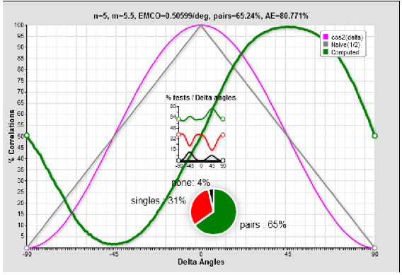
Each polarizer is related to a rate of detections, also called arm efficiency ( AE). The general efficiency or cross efficiency is the pairs rate of the 2 polarizers, in general the product of the 2 arms efficiencies.
With this first simulated curves comparison, the efficiency by arm is 84.9%, of the same order as the best detectors currently in the market. In the lab, the efficiency objectively reported in the greatest experiments [4] is lower. When the efficiency is summed on the raw data, before the lab experiment data filtering, the rates are 1 to 3 orders lower. That the lab filters the data in a fundamental experiment is beyond the scope of this article.
Observe that the green and magenta curves are almost superposed with different values of the m and n crystal parameters.
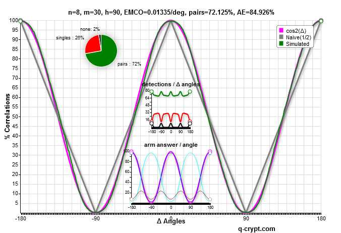
The functions vary smoothly with the change of the n and m parameters. m can be real but n must be an integer.
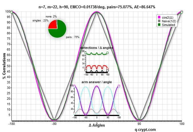
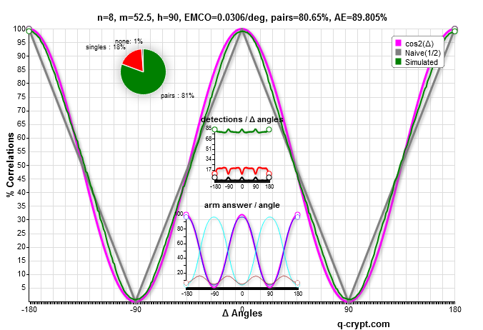
These 4 curves are the most efficient respectively for n=8,7,6 and 5.
the parameters setting n=6 and m=6.5 gives the most similar to the cos² curve.
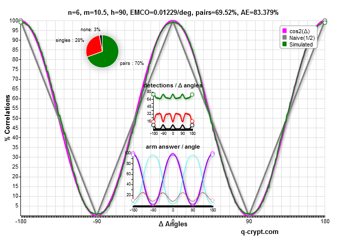
It seems that n=5 and m=5.25 is the more similar to the lab correlation curve, with less fitting at extreme values.
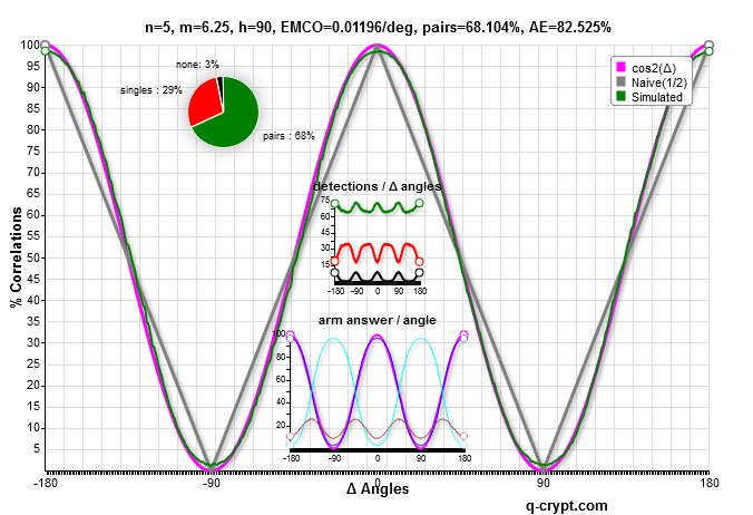
We can choose the m and n parameters to get more detections at the price of more differences between the curves.
When m becomes high , the efficiency raises until 99% and the curve is this time similar to the classical reference. Specific labs experiments, exploring the variations of n and m, may question the physicality of the distribution.
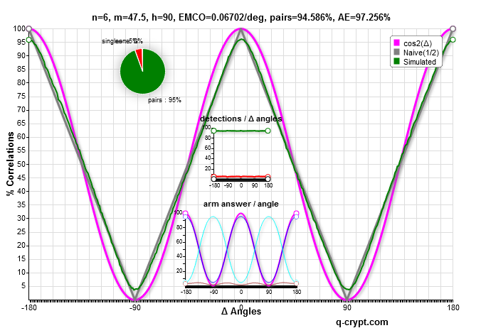
Is the curve below acceptable as quantum like ? probably yes. A 90% efficiency detector doesn’t yet exist.
4.3 Observations and physicality
4.3.1 Limits
-
-
-
- The shared variable cannot be static and must be distributed in a radius \(\rho\) from \({\pi \over 4}\) to \(\pi \over 2\) around zero. However, the distribution by arm is constant with a \(\pi \over 2\) radius while it is near of the Malus law with \(\pi \over 4\). The latter is retained as a constant in this paper. But it is possible to get another value based on lab arm measures showing a detection rate depending on the angle.
- Using a gaussian shared variable, while it might have a physical meaning, does not have an impact on the shapes of the resulting curves.
- n must be a positive integer while m may be a positive real.
-
-
4.3.2 Similarity
The original analyse predicts the exact correlation curve when the errors and undetections rates are null. But, pratically, there are errors and, as it is shown, a classical algorithm can render the same results in the final statistics. Adjusting the parameters to get a 100% detection gives the original Bell classical correlation curve, which is a particular case of the cross distribution.
Numerical searches of optimal m and n were done on a computers network. The best fitting is around 68%. Is it rather \(2 \over 3\) with a perfect curve superposition? The best cross efficiency with a curve yet very similar to cos² is 75%. Fitting and efficiency are in balance.
We found better formula based on hypotetic walks of a photon in a crystal with simple exit rule. They need more computation capacity, then they cannot be checked within a browser on the internet as this markovian distribution.
4.3.3 systematic check, if it was the clock and the phase
It is interesting in a classical Bell experiment to do some quick checks to discard trivial classical results.
The shared variables sequence may come from a clock. In optical settings, one can question the physicality of h in the phase shared by 2 coherent photons by checking a statistics of coherent photons not explicitely entangled. Then, 2 flows of almost coherent photons coming from 2 sources must correlate in cos² if the distribution is physical and the shared variable the phase.
Let’s assume that h is no more a shared variable and is replaced by h1 and h2 such h2-h1 = constant.
The MC computation shows now the same corresponding phase in the correlation curve! Above, h1 and h2 have a constant difference of \(\pi/4\) which is the same as the shift of the correlation function.
Giving a small random difference to h2-h1 weaken the efficiency but the curve is still similar to cos². Then, 2 flows of mere coherent photons coming from 2 stable sources don’t need to be perfectly adjusted to execute this experiment.
If it is exactly the phase, a photons sequence from a coherent light might also correlate with itself, by using 2 paths of different lengths.
Unfortunately, these systematic checks will probably be negative. This doesn’t invalidate the computability of such correlations and the need of a high luminosity to prove any interpretation.
4.3.4 From where came the classical curve used by Bell?
A classical analysis without detections errors shows that correlations behave like in QM but with 50% of noise. Normally after this step, it seems obvious to evaluate better variants than the naive Malus application, in the same way it is done for refractions at the quantum level [5], and to invoke intrinsic errors in the measures. These 2 hypotheses are enough to make the Bell inequality useless in a lab, unless an undreamed resolution technology arises.
5. About a proof of quantum entanglement using the Bell Settings
- It is now a fact that, in lab conditions of experimentation, classical possible distributions very similar to cos² exist and cannot be ignored.
Therefore, to be conclusive an experiment must show properties that a local computation cannot do. It is still possible with the same setting if the measured curve is similar to cos² with very small differences and if the observed real efficiency is largely above 75% or wathever high value established by a fine analysis after the search and the check of other distributions candidates. It is not yet done.
6. Conclusion
6.1 Bell theorem
Hence, a new Bell theorem must now include an explicite condition on the raw detection rate to be experimented in a lab.
6.2 Classical Pseudo-Entanglement
An interesting point is the production by software of classical pseudo-entangled signals, not yet enough to encrypt or compute as currently theorized but useful in many other contexts. It leads to other encoding methods and opens the mind about artifacts. The usual no-GO theorems don’t apply on classical pseudo-entanglement then it is possible to pseudo-entangle classically any pair of many “polarizers” sharing the same variables sequence. This can give many ideas, knowing that their data are all random and independent. However, we can show that this encrypting cannot resist to specific algorithms like our A51*. Using physical correlations which cannot be quantum entangled leads finally to a too expensive weak-encrypting.
6.3 Quantum Mechanics and interpretations
We were asked if it was a claim of the invalidity of the quantum entanglement and then of the Copenhagen interpretation. Yes, it was. Copenhagen interpretation has not yet any experimental fundament. It is still a speculative assumption which needs to be proven or abandoned.
Each experiment claiming that it is conclusive must be checked again. The efficiencies of the detectors, polarizers and optical devices are given by the constructors. A whole detection rate is the product of those of all components, so it is less than the smallest of them. Pre and post selections leads again to classical.
It is easy to predict the outcomes of these reanalyses.
6.4 Experiments
The versality of the above distribution and its apparent physicality are intriguing, to say the least. We would be glad to participate to an experiment with or without many referees. It would include the measure of the relation between the quality and the detection rate and check some possible sources of shared variables, not only the phase.
A Supplemental material
A.1 Other functions
When the photon walk in a crystal is simulated by more Monte-Carlo distributions at the lowest level, the efficiency tends to \(2 \over 3\) while the differences with cos² become very smaller than the ones seen above. The markovian simplification seems to reduce the noise. However, it produces pseudo-entangled sets quickly and allows online checks, something impossible else. Large trials of these slow functions had been made in 2013 and produced a lot of data. Another family of distributions tends in the same way to \(2^{-{1 \over 2}}\).
We think that the search of the good distribution cannot be driven by aesthetic, nor by a principle of minimalization since there are so many. Interpretations must come only after a rigorous experiment.
A.2 Softwares
The scripts for the deep MC version are written in C++.
Another version simulates 4 independent agents running their scripts independently, the shared variable oracle, the 2 polarizers and the final stage. When they meet to establish the statistics, they find obviously the same results as if all was computed by the same box…
A.3 Share
Most softwares and data may be shared or are already public. Get in touch with the author to get other specific links or a help for a specific port.
*: we will make it public on demand.
References
1 J. S. Bell (1964) : On the Einstein-Podolsky-Rosen Paradox, Physics 1, 195-200 . and pdf
3 A. Aspect : Bell’s Theorem : The Naive View of an Experimentalist (2002). and Arxiv
4 Marissa Giustina, Alexandra Mech, Sven Ramelow, Bernhard Wittmann, Johannes Kofler, Jörn Beyer, Adriana Lita, Brice Calkins, Thomas Gerrits, Sae Woo Nam, Rupert Ursin, Anton Zeilinger (2013) : Bell violation with entangled photons, free of the fair-sampling assumption Nature 10.1038/nature12012 and Arxiv .